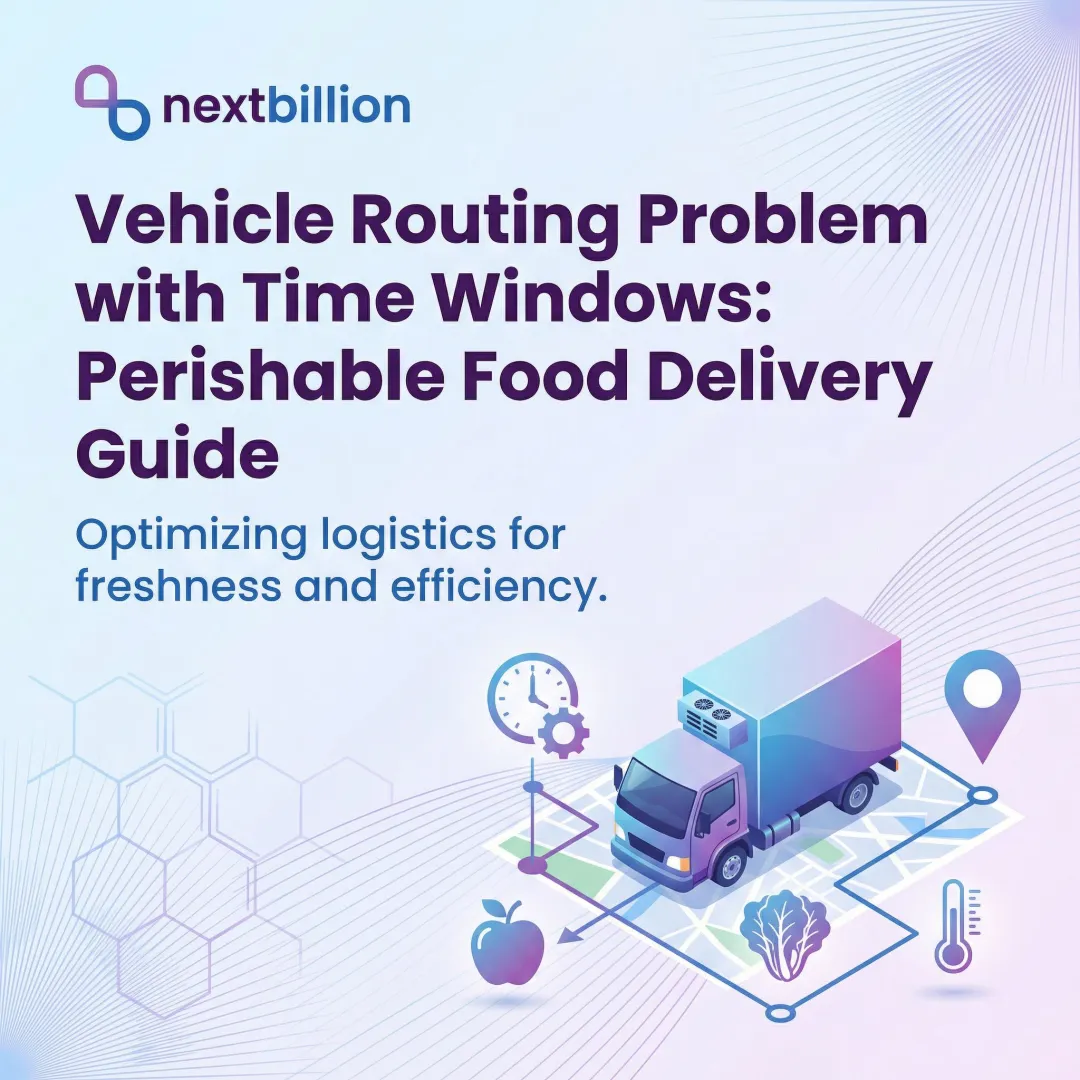
Introduction
Real-world logistics rarely unfolds as planned. New orders arrive after drivers depart, traffic grinds routes to a halt, vehicles break down, and customers change their availability. By noon, a carefully optimized morning plan can be unworkable. Dynamic Vehicle Routing with Time Windows (DVRPTW) addresses this by extending classic route optimization into a continuous, real-time framework where vehicles must visit customers within specified time slots while adapting routes as conditions shift mid-operation.
For logistics and transportation operators—whether in last-mile delivery or field service scheduling—missing time windows directly hits costs, customer satisfaction, and fleet utilization. Failed first-attempt deliveries can add up to 15–20% in additional operational expenses through re-routing, wasted driver time, and lost customers.
DVRPTW is the operational answer: a routing framework that maintains time window compliance while absorbing the disruptions inherent in live operations.
What follows covers how dynamic VRPTW differs from static routing, how the process works end-to-end, which factors shape performance, and where applying it may be unnecessary or counterproductive.
TLDR
- DVRPTW optimizes routes that respect customer time windows AND adapts in real time to new orders, cancellations, or disruptions
- Unlike static VRPTW—solved once before dispatch—DVRPTW re-optimizes continuously as conditions change mid-operation
- Hard time windows (strict deadlines) vs. soft windows (flexible with penalties) — each demands a different solver approach
- Performance depends on fleet size, demand patterns, window tightness, solver latency, and constraint complexity
- Not every operation needs dynamic VRPTW—stable, pre-scheduled routes see little benefit from real-time re-optimization
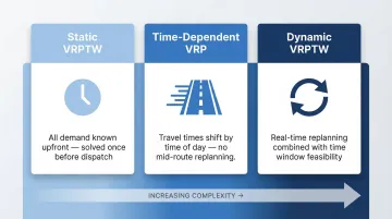
What Is Dynamic Vehicle Routing with Time Windows?
DVRPTW is a variant of the Vehicle Routing Problem where a fleet of vehicles must serve geographically dispersed customers, each with a designated time window for service, while the set of customers, locations, or constraints can change during plan execution. The goal: minimize total travel cost or time while ensuring every customer is visited within their allowed time window and the routing plan remains viable as conditions evolve.
Distinguishing DVRPTW from Related Problems
Three related problem variants are easy to conflate:
- Static VRPTW: All demand is known upfront; routes are solved once before dispatch
- Time-dependent VRP: Travel times shift by time of day (peak-hour congestion), but routes aren't re-planned mid-execution
- DVRPTW: Combines real-time replanning with time window feasibility, making it operationally distinct from both
Hard vs. Soft Time Windows
Two time window types appear across DVRPTW implementations:
- Hard time windows: Early arrival means waiting; late arrival is infeasible. The academic and operations literature from Solomon (1987) onward has predominantly benchmarked against hard windows
- Soft time windows: Violations are allowed at a penalty cost—computationally easier but requiring careful penalty calibration
Constraint Windows vs. Solution Windows
A constraint window is the customer's stated availability slot (for example, 2:00 PM - 4:00 PM). A solution window is the tighter feasible arrival interval computed by the solver based on travel times and route sequencing—often smaller than the constraint window due to cumulative time propagation along the route.
Why DVRPTW Matters in Modern Logistics
Operational Pressure Driving DVRPTW Adoption
Real-world logistics rarely unfolds as planned. New orders arrive after dispatch, traffic delays cascade, vehicles break down, and customer time preferences vary. Static routing is insufficient for operations that must stay efficient under uncertainty—especially when time window compliance is non-negotiable.
Domains Where DVRPTW Is Critical
Time window compliance is non-negotiable across several high-stakes domains:
- Same-day e-commerce delivery
- On-demand food delivery platforms
- Non-Emergency Medical Transportation (NEMT) with appointment constraints
- Field service technician dispatch
- Last-mile pharmaceutical distribution
Each carries hard service commitments that cannot be violated without financial or regulatory consequences. Without dynamic time window routing, the consequences compound quickly.
The Cost of Static Routing
Drivers accumulate late arrivals, failed deliveries require costly re-attempts, and fleet capacity is wasted on inefficient sequencing. Failed first-attempt delivery rates can reach 15–20%, directly inflating costs through duplicate trips and driver overtime.
The Business Case for DVRPTW
DVRPTW delivers measurable ROI beyond regulatory compliance. The business case centers on:
- Reducing kilometers driven
- Reducing idle time and driver overtime
- Absorbing demand surges without adding vehicles
- Improving on-time delivery rates
For operations running at scale, these gains compound — fewer vehicles needed, lower fuel spend, and stronger delivery reliability that directly influences customer retention.
How Dynamic VRPTW Works
DVRPTW is not a one-time solve but an iterative loop. An initial route plan is generated pre-dispatch using known orders, and as the day progresses, new events trigger partial or full re-optimization of open routes, with solvers finding the best feasible insertion or rerouting within tight time constraints.
Data Inputs Required
The process requires:
- Time matrix (travel times between all location pairs, may vary by time of day)
- Time windows per customer (earliest and latest service times)
- Vehicle capacities and fleet size
- Service durations at each stop
- Real-time event feed for new orders or cancellations
Phase 1: Initial Route Construction
Before dispatch, a construction heuristic—such as nearest feasible neighbor insertion or savings-based algorithms—builds an initial feasible route set that satisfies all known time windows and capacity constraints. This forms the baseline solution from which dynamic updates depart.
Insertion heuristics are highly advantageous for VRPTW because tight time windows naturally constrain potential customer placements, drastically reducing the number of feasible insertions that must be evaluated and speeding up the solution process.
Phase 2: Real-Time Event Handling and Re-Optimization
As new service requests arrive or disruptions occur mid-route, the solver must decide whether to insert the new customer into an existing route (cheapest feasible insertion), open a new route, or defer the request—each decision constrained by the time windows of existing customers already committed to active routes.
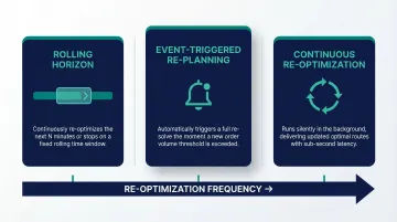
Re-solve strategies used in practice:
- Rolling horizon approaches: Only re-optimize routes for the next N minutes/stops
- Event-triggered re-planning: Re-solve when a threshold number of new orders arrive
- Continuous re-optimization: Solve in the background with sub-second latency
The cheapest insert search allows systems to rapidly evaluate new orders against the current schedule in memory, accepting or rejecting customers based on the availability of a feasible, cost-effective insertion point. The cheapest insert search allows systems to rapidly evaluate new orders against the current schedule in memory, accepting or rejecting customers based on the availability of a feasible, cost-effective insertion point.
In production deployments, platforms like NextBillion.ai's Route Optimization API support 50+ hard and soft constraints to enable practical real-time re-solve across large fleets.
Phase 3: Constraint Propagation and Feasibility Enforcement
Solvers maintain a dimension tracking cumulative travel time at each node. If a vehicle's arrival at any node would violate that node's time window, the route is infeasible and must be rescheduled or a penalty applied.
This constraint propagation is what makes VRPTW significantly harder than unconstrained VRP. State-of-the-art exact solvers rely on column generation, where the pricing subproblem is modeled as an Elementary Shortest Path Problem with Resource Constraints (ESPPRC).
Because ESPPRC is strongly NP-hard, solvers use pseudo-polynomial labeling algorithms combined with strict dominance rules and k-cycle elimination. Together, these techniques prune infeasible paths and keep the exponentially growing search space manageable.
Key Factors That Affect Dynamic VRPTW Performance
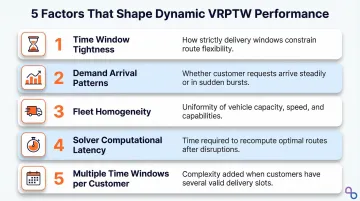
DVRPTW performance depends on both algorithmic design and real-world operational conditions. These five factors carry the most weight:
- Time window tightness: Narrow windows shrink the feasible solution space, increasing solve difficulty and the likelihood of needing to drop or delay customers
- Demand arrival patterns: Clustered versus random demand affects whether re-optimization yields meaningful improvements or simply adds computational overhead
- Fleet homogeneity: Mixed fleets with different capacities, speeds, or vehicle restrictions (e.g., truck routing with weight/height limits) multiply the constraint surface and require vehicle-specific subproblem solving
- Solver computational latency: In dynamic contexts, a solution returned in 30 seconds may be outdated; sub-second or low-latency solvers are operationally necessary for high-frequency re-planning
- Multiple time windows per customer: Some customers specify several acceptable service slots (VRPMTW), adding combinatorial complexity while better reflecting real-world availability — for example, businesses with split operating hours
Common Misconceptions About Dynamic VRPTW
These misconceptions typically stem from treating related-but-distinct concepts as interchangeable. Each one leads to real implementation problems — misconfigured solvers, unstable routes, or incomplete problem formulations.
VRPTW and Dynamic VRPTW Are Not Interchangeable
Static VRPTW assumes complete, fixed demand information and solves once before execution. Dynamic VRPTW is defined by incomplete or changing information during execution — the two variants require fundamentally different solver designs, not just different inputs to the same algorithm.
More Frequent Re-Optimization Doesn't Always Help
Excessive re-planning introduces route instability — drivers receive conflicting instructions mid-route, customers get uncertain arrival windows, and computational resources get consumed with diminishing returns. Effective DVRPTW implementations apply re-optimization selectively, triggered by defined thresholds rather than every new event.
Time-Dependent Travel Times vs. Time Windows
Time-dependent VRP adjusts arc travel costs based on the time of day — for example, routing around peak-hour congestion. Time windows, by contrast, constrain when a customer can be visited, regardless of travel conditions. These are separate mechanisms. Treating them as the same thing typically produces formulations that handle congestion but ignore delivery slots, or vice versa.
When Dynamic VRPTW May Not Be the Right Approach
Operations with Stable, Pre-Booked Demand
DVRPTW is unnecessary for operations with stable, pre-booked demand—such as fixed milk-run routes or school bus routing with set schedules. These operations derive little value from dynamic re-planning because the problem is effectively static and solved optimally pre-dispatch. Adding a dynamic layer introduces complexity without operational benefit.
Constraints That Reduce DVRPTW Effectiveness
Time window structure directly limits how much dynamic optimization can deliver:
- Extremely wide windows (several hours or more) reduce the benefit because almost any reasonable stop sequence is feasible — the algorithm has little to improve.
- Extremely tight windows where only one feasible sequence exists per route give dynamic re-planning no room to maneuver, so re-optimization rarely changes the outcome.

Signals DVRPTW Is Applied by Default, Not Need
Two operational signals suggest DVRPTW is being applied by default rather than genuine need:
- Re-optimization consistently produces the same routes as the initial plan — meaning disruptions aren't actually occurring.
- Driver compliance with updated instructions is low, making re-plans ineffective regardless of how good the algorithm is.
Either pattern indicates the operation lacks the demand uncertainty or disruption frequency that warrants the added complexity.
Conclusion
Dynamic VRPTW extends classical time-window-constrained routing into an adaptive, real-time framework that keeps fleet operations feasible and efficient as demand, traffic, and operational conditions evolve throughout the day. For logistics environments where time commitments are non-negotiable and disruptions are constant, it's the formulation that actually holds up in production.
Understanding the distinction between static VRPTW, dynamic VRPTW, and related variants matters for operations teams. Selecting the right formulation and solver capability — matched to actual demand volatility, time window structure, and fleet complexity — is what separates operationally effective route optimization from theoretical compliance.
Not every operation needs dynamic VRPTW. But for those that do, getting the solver and constraint model right determines whether you're consistently hitting delivery windows or absorbing the cost of failed attempts and reroutes. Teams evaluating route optimization APIs should specifically probe for real-time re-optimization support, constraint depth, and response latency — these are the capabilities that make dynamic VRPTW work at scale, not just in theory.
Frequently Asked Questions
What is the vehicle routing problem with time windows?
VRPTW is a combinatorial optimization problem where a fleet of vehicles must serve a set of customers, each with a defined earliest and latest service time (time window), while minimizing total travel cost or time. If a vehicle arrives early it must wait; late arrivals are either infeasible (hard windows) or penalized (soft windows).
What is the time dependent vehicle routing problem?
The time-dependent VRP is a variant where travel times between locations vary based on the time of day (e.g., peak-hour congestion), meaning the cost of traversing an arc depends on when a vehicle departs. This differs from VRPTW, where the constraint is on when a customer can be served, not on how long it takes to travel there.
What is the dynamic park and loop routing problem?
The dynamic park-and-loop problem involves a vehicle parking at a central point and a courier completing a loop on foot or by bicycle to serve nearby customers, with the vehicle repositioning dynamically as demand shifts. It is used in dense urban last-mile delivery and inherits VRPTW-style time constraints at the customer level.
What is the difference between hard and soft time windows in vehicle routing?
Hard time windows are strict constraints—arriving outside the window renders the solution infeasible. Soft time windows allow violations at a penalty cost incorporated into the objective function. Soft windows are computationally easier to handle but require careful penalty calibration to reflect real operational consequences.
How does dynamic VRPTW handle new customer requests that arrive after dispatch?
New requests are checked for feasible insertion into existing routes using cheapest insertion heuristics. If no feasible slot exists without violating committed time windows, the solver may open a new route, defer the request, or flag it for human review, depending on the solver's re-optimization trigger and latency capabilities.
What algorithms are commonly used to solve large-scale dynamic VRPTW problems?
Heuristic and metaheuristic methods dominate in practice—including adaptive large neighborhood search (ALNS), variable neighborhood search (VNS), and increasingly reinforcement learning-based approaches. Exact methods such as branch-and-price become computationally intractable beyond small instance sizes, making scalable heuristics the operational standard for real-time re-optimization.