Introduction
Every morning, delivery fleets start their routes armed with precisely optimized schedules—routes optimized to the minute. But within hours, reality strikes. A driver hits rush-hour gridlock on a normally free-flowing highway. The 12-minute segment now takes 28 minutes. The cascade begins: the next stop runs late, pushing the third delivery past its time window. By afternoon, the fleet faces missed commitments, driver overtime, and reactive rescheduling that erodes both margins and customer trust.
This isn't a failure of planning discipline. It's the fundamental flaw of static routing in a dynamic world. Peak-hour travel times are 60–80% longer than off-peak conditions, yet most routing systems treat travel time as a fixed constant. The result? Static routing wastes 15–22% of fuel and consistently underestimates route duration, triggering cascading operational failures.
This article breaks down why static routing fails under real-world conditions, how dynamic travel time modeling works, and what to look for in a route optimization platform built for it.
Why Static Routing Fails in the Real World
Traditional Vehicle Routing Problems (VRP) rest on a computationally convenient but operationally dangerous assumption: travel time between any two stops is a fixed constant, typically derived from free-flow speeds or historical averages. This assumption greatly simplifies mathematical complexity, allowing solvers to treat every route segment as predictable. But roads don't work that way.
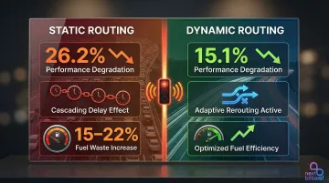
When static plans collide with dynamic roads, feasibility collapses. Routes that appear viable during planning become infeasible the moment a vehicle enters peak-hour congestion. Research shows that even 10% reductions in average speed cause significant route overruns, with drivers routinely exceeding planned duty hours and missing customer commitments. In extreme traffic variability, static routing suffers performance degradation of 26.2%—nearly double the 15.1% degradation experienced by dynamic systems operating under identical conditions.
That first late stop rarely stays isolated. One delayed stop shifts all downstream time windows, creating constraint violations that ripple through the entire route. The third customer misses their window because the second stop ran 20 minutes over, the driver exceeds hours-of-service limits, and dispatch scrambles to reassign stops—fragmenting the original plan and compounding both driver stress and operational costs.
Many planners respond with the "contingency allowance" workaround—uniformly reducing assumed speeds by 10–20% across all segments and time periods. This blunt instrument forces a difficult trade-off:
- Too little buffer: Routes stay infeasible during peak periods, and delays repeat
- Too much buffer: Fleets get over-provisioned with unnecessary vehicles and idle capacity, wasting labor and capital while limiting service coverage
Static routing also ignores the emissions dimension. Vehicles traveling at congested, stop-and-go speeds consume vastly more fuel per mile than vehicles at moderate steady speeds. Aggressive stop-and-go driving in traffic can lower fuel efficiency by 10–40%. For a fleet running dozens of routes daily, routing trucks into predictable congestion adds measurable fuel costs and emissions on top of every missed time window.
Understanding Dynamic Travel Times in Vehicle Routing
Dynamic travel times mean travel duration on any road segment is a function of departure time, not a fixed value. Instead of assuming the trip from Stop A to Stop B always takes 15 minutes, time-dependent routing recognizes that leaving at 8:00 AM during peak congestion takes 24 minutes, while leaving at 10:30 AM takes just 12 minutes.
This requires time-dependent speed profiles—discrete time buckets (typically 5- to 15-minute intervals) where speed on each road segment changes according to observed congestion patterns. Commercial traffic APIs from providers like TomTom and Mapbox structure historical speed data this way, enabling routing engines to query: "What is the expected speed on this segment if I depart at 8:15 AM?"
Any valid time-dependent model must satisfy the FIFO (First-In, First-Out) property: if a vehicle departs a location at time T₁, an identical vehicle departing at T₂ > T₁ must arrive no earlier than the first vehicle.
FIFO prevents scenarios where delaying departure paradoxically results in earlier arrival—a mathematical artifact that plagued early step-function models and made them operationally unreliable.
Predictable vs. Unpredictable Dynamics:
- Predictable dynamic travel times reflect recurring patterns—rush-hour slowdowns, midday traffic easing, weekend vs. weekday differences—captured from historical speed observations. Most commercial routing solutions primarily address this predictable component.
- Unpredictable dynamic events include accidents, weather disruptions, and real-time incidents. Handling these requires real-time traffic feeds and mid-execution re-optimization, which adds complexity beyond historical modeling.
Time-dependent routing extends the classic VRPTW (Vehicle Routing Problem with Time Windows): each customer must be visited within a specified time window, and travel time between any two customers now depends on when the vehicle departs the first location. This interdependency expands computational complexity significantly: every routing decision shifts departure times for subsequent stops, which cascades through all downstream travel times.
Path Flexibility Matters
In real road networks, multiple physical paths connect any two locations. At different departure times, different paths become optimal. A highway route that's fastest at 10 AM may become congested at 5 PM, making a surface-street alternative faster, cheaper, or lower-emission. Time-dependent routing must evaluate not just when to travel, but which path to take at that time.
Data Requirements
Implementing time-dependent routing demands reliable speed data at the road-segment level across time periods. This requires:
- GPS-sourced historical speed observations aggregated by time of day and day of week
- Real-time traffic APIs for current conditions
- Road network models that map physical segments to time-dependent cost functions
Without this granularity, the optimizer is essentially guessing—and those guesses compound across every stop in a multi-vehicle schedule.
Key Challenges in Dynamic Vehicle Routing and Scheduling
Computational Complexity
The static VRP is already NP-hard (a problem class where solution time grows exponentially with problem size). Adding time-dependence dramatically expands the solution space. Every routing decision alters departure times for all subsequent stops, which changes travel times, which affects feasibility of time windows, which influences the next routing decision.
Research shows that in time-dependent graphs with piecewise linear edge costs, arrival time functions can have a superpolynomial number of breakpoints, making exact solutions computationally prohibitive for real fleet sizes. Heuristic and metaheuristic methods, including Adaptive Large Neighborhood Search (ALNS), Tabu Search, and Ant Colony Optimization, dominate practical applications because they find near-optimal solutions within acceptable timeframes.
Constraint Interdependency
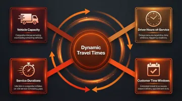
Dynamic travel times interact with every other routing constraint in unpredictable ways:
- Vehicle capacity: A route that's capacity-feasible under static times may become infeasible if congestion delays cause perishable goods to spoil or refrigeration limits to be exceeded
- Driver hours-of-service: Longer-than-planned travel times push drivers past legal duty limits
- Customer time windows: Even small delays cascade, making downstream windows unreachable
- Service durations: Fixed stop times consume a larger proportion of available time when travel takes longer
A local improvement that benefits one route (like swapping two stops) can ripple through timing dependencies and render another route infeasible. Verifying feasibility becomes harder, and solution quality depends on the solver's ability to evaluate these interdependencies efficiently.
Real-Time Re-Optimization
Mid-execution disruptions demand immediate replanning. When a new order arrives, a road incident occurs, or a service stop takes longer than expected, the entire active route plan must be re-evaluated. The "degree of dynamicity" measures what percentage of orders or conditions are unknown at planning time. Real-world urban delivery simulations show an average of 27.4 disruptive events per scenario. Higher dynamicity demands faster re-optimization engines that can handle partial route commitments—stops already in progress or completed cannot be reassigned, constraining the feasible solution space for updates.
Balancing Service Rate and Operational Efficiency
That pressure for faster replanning connects directly to a deeper operational tension: maximizing customers served (service rate) versus minimizing total cost (vehicle time, fuel, driver wages). Fleet managers live at this intersection every day.
Aggressively packing stops into routes boosts service rate but increases infeasibility risk under real traffic conditions — vehicles can't physically complete the route within time windows or duty limits. Over-conservative planning wastes capacity and limits growth. Time-dependent routing sharpens this trade-off by revealing which routes are genuinely feasible and which are built on optimistic assumptions.
Approaches and Algorithms for Dynamic Route Optimization
Modern dynamic routing engines rely on a family of practical algorithms designed for speed and solution quality within tight operational constraints:
Construction Heuristics and Local Search:
- Time-dependent nearest-neighbor heuristics build initial solutions by iteratively selecting the next stop with the lowest time-dependent travel cost from the current position
- Local search operators like 2-opt, cross-exchange, and or-opt are adapted to evaluate moves using time-dependent cost functions, swapping stops or reversing route segments to find improvements
- The most effective solvers combine multiple methods—fast construction for initial feasibility, then local search for refinement within seconds
Metaheuristics for Complex Scenarios:
- Adaptive Large Neighborhood Search (ALNS): Repeatedly destroys and rebuilds portions of the route plan, which lets it escape local optima that simpler solvers get stuck in
- Tabu Search: Tracks recently visited solutions in a memory structure to prevent cycling, steering the search toward unexplored, potentially better configurations
- Ant Colony Optimization (ACO): Virtual "ants" construct routes probabilistically; paths that consistently yield shorter travel times get reinforced across iterations, converging on strong solutions

Knowing which algorithms to apply is one part of the problem. The other is knowing when to apply them—which is where the rolling time-slice approach comes in.
Rolling Time-Slice Approach:
For real-time dynamic routing, the working period is divided into discrete time slices. At each slice:
- Newly available orders are inserted into the plan
- Stops already committed or in progress are locked
- Remaining open stops are re-optimized
This converts the continuous dynamic problem into a series of tractable static sub-problems that can be solved incrementally. Research shows that a replanning interval 10–15 minutes shorter than the planning horizon optimally balances computational load, route stability, and responsiveness.
Warm-Starting and Pheromone Preservation:
Instead of restarting optimization from scratch when new events arrive, advanced solvers carry forward learned route quality information from the previous solution as a starting point. This approach—called "warm-starting" or "pheromone preservation"—cuts computation time while still producing near-optimal updates.
In practice, this means a solver handling a new vehicle breakdown or late order can recalculate affected routes in seconds rather than re-running the full optimization cycle, keeping dispatchers and drivers aligned without interruption.
Measuring the Business Impact: Costs, Emissions, and On-Time Performance
Direct Operational Costs
Ignoring dynamic travel times creates measurable, avoidable waste. Research quantifies that static routing wastes 15–22% of fuel by failing to account for real-time traffic dynamics. Routes consistently exceed planned duration, triggering overtime labor costs that erode margins.
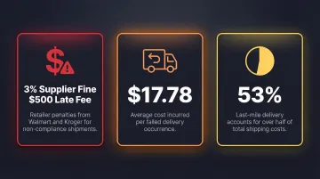
The downstream penalties compound quickly:
- Walmart charges suppliers 3% of the purchase price for late deliveries; Kroger fines $500 for orders more than two days late
- Failed deliveries cost an average of $17.78 per occurrence, doubling driver time, fuel, and vehicle wear for a single stop
- Last-mile delivery already accounts for 53% of total shipping costs—routing inefficiency compounds an already expensive problem
Emissions Benefit
Time-dependent routing that avoids congested periods and selects paths based on actual speed profiles reduces fuel consumption. Vehicles spend less time at low-efficiency stop-and-go speeds, cutting both cost and emissions. Advanced time-aware routing methods can increase on-time delivery rates from 68.1% to 92.8% while reducing operational costs by 24.3% and cutting congestion exposure by 54.4%.
On-Time Delivery Rate
On-time delivery is the key customer-facing metric. Dynamic routing reduces missed time windows, lowers complaint rates, and protects revenue. For food delivery, NEMT, or field services—where time windows are contractual or safety-critical—missing a window often means losing the customer entirely.
Consistent on-time performance builds the kind of reliability that drives repeat business. Carriers that slip below acceptable delivery rates with major retail partners can lose shelf placement altogether, making routing accuracy a revenue protection issue, not just an operational one.
What to Look for in a Dynamic Route Optimization Solution
Data Integration at Scale
A capable platform must ingest real-time and historical traffic data at the road-segment level, not just city-level averages. Look for support for large distance matrices computed with time-dependent travel times. Many routing APIs impose artificial limits—Google Maps caps distance matrices at 25×25, forcing workarounds that degrade optimization quality. Enterprise-grade solutions should support matrices of 1,000×1,000 or larger, enabling full-fleet optimization without artificial segmentation.
Constraint Richness
Dynamic travel times are just one dimension. A production-grade solution must simultaneously handle:
- Vehicle capacity and load constraints
- Driver hours-of-service regulations
- Customer time windows (hard and soft)
- Service durations and setup times
- Priority tiers and customer preferences
- Multi-stop sequencing and pickup-delivery pairing
- Vehicle-specific restrictions (truck size, weight, hazmat)
Solutions with limited constraint sets force planners into manual workarounds that reduce optimization quality and increase operational complexity. The best platforms support 50+ hard and soft constraints, enabling realistic schedules that reflect actual business rules.
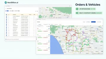
NextBillion.ai: Built for Enterprise-Scale Route Optimization
NextBillion.ai's route optimization platform supports 50+ hard and soft constraints alongside time-dependent routing, enabling fleets to plan schedules that account for traffic patterns, vehicle restrictions, driver regulations, and customer requirements — all at once.
Its API-first architecture integrates directly into existing TMS, dispatch systems, and fleet management platforms—including Samsara, Geotab, Motive, and Netradyne—without requiring infrastructure overhaul. Routes flow directly from optimization engine to driver app, eliminating manual re-entry and the errors that come with it.
Beyond the API, several operational factors set the platform apart:
- Per-vehicle pricing — unlike per-API-call models, costs stay predictable even with thousands of daily re-optimizations across large fleets
- Flexible deployment — supports on-premise, Kubernetes, and cloud-agnostic environments for teams with data residency or latency requirements
- Compliance coverage — SOC 2 Type II, GDPR, CCPA, and ISO/IEC 27001:2013 certified for regulated industries
Frequently Asked Questions
What is the difference between static and dynamic vehicle routing?
Static routing assumes fixed travel times between stops, treating roads as unchanging regardless of time of day. Dynamic routing accounts for travel times that vary based on departure time, traffic congestion, and real-world road conditions, producing more reliable and efficient schedules for actual operations.
What is a time-dependent vehicle routing problem (TDVRP)?
TDVRP is a variant of the classic vehicle routing problem where travel time between any two locations depends on when the journey begins, reflecting time-varying traffic speeds. Solving it requires algorithms that account for how departure time at each stop affects all downstream travel times and route feasibility.
How does traffic congestion specifically affect delivery scheduling?
Congestion pushes actual travel times past plan estimates, causing downstream stops to start late, time windows to be missed, and driver duty periods to be exceeded. The result is reactive rescheduling, overtime costs, and customer service failures that compound expenses and erode reliability.
What algorithms are commonly used for dynamic vehicle routing?
Common approaches include Ant Colony Optimization, Tabu Search, and hybrid metaheuristics paired with time-dependent construction heuristics and local search operators. In production, the most effective systems use warm-started re-optimization within rolling time windows to respond to real-time events quickly.
Can dynamic route optimization reduce fuel costs and emissions?
Yes. By routing vehicles through paths and at times that avoid stop-and-go congestion, dynamic optimization reduces idle time and low-efficiency driving. Research indicates this can yield fuel consumption reductions of 15–22% and measurable CO₂ reductions compared to static planning methods.
How do you handle new orders or route disruptions in dynamic routing?
Modern dynamic routing systems use rolling re-optimization: when a disruption or new order arrives, in-progress stops are locked and the remaining schedule is re-optimized in near real-time — balancing continuity with responsiveness.