The Dynamic Vehicle Routing Problem (DVRP) under traffic congestion is fundamentally different from classic VRP. Routes aren't planned once and executed—they must be continuously re-evaluated as conditions change. Travel times shift, new orders arrive, and congestion states evolve unpredictably throughout the day.
This article explains why traffic makes routing computationally hard, what solution approaches researchers and operators actually use, and what to demand from modern routing technology that claims to solve this problem.
TL;DR
- DVRP under traffic congestion requires real-time route re-optimization because travel times change dynamically and unpredictably
- The solution is a policy (decision rules), not a fixed route sequence
- Key approaches include MDP models, learnheuristics (ML combined with metaheuristics), agile optimization, and rollout algorithms
- Traffic-blind routing inflates fuel costs by 13% and consistently causes missed delivery windows
- Modern route optimization APIs embed real-time congestion data and sub-second re-routing to keep routes accurate as conditions shift
What Makes Dynamic Vehicle Routing Under Traffic Congestion Fundamentally Different
Unlike static VRP where all inputs are known before departure, the DVRP involves information that evolves in real time—new orders, cancelled stops, and critically, travel times that change due to traffic congestion.
Why Traffic Congestion Is Uniquely Disruptive
Travel time between two nodes is neither fixed nor proportional to distance in urban environments. A 2-km arc through city center at 8:30 AM may take 3× longer than the same arc at 10:00 AM.
Research confirms that "when travelling between two random centroids in any city, the distance over the urban road network is on average 41% greater than the distance travelled in an ideal straight line." Euclidean distance assumptions break down entirely.
More importantly, each arc consists of multiple road segments with their own speed distributions. Modeling an arc as a single travel time doesn't work: you need to decompose it into individual road segments and estimate each segment's speed distribution separately.
The Curse of Dimensionality
As nodes and traffic states increase, the solution space grows exponentially. The number of arcs always exceeds the number of nodes, so traffic-sensitive routing tracks far more states than demand-only models. Exact dynamic programming faces the "three curses of dimensionality": vast state space, action space, and stochastic information space.
Time-dependent vs. stochastic travel times:
- Time-dependent (deterministic): Congestion follows a predictable daily pattern (e.g., rush hour)
- Stochastic: Travel times are random variables even within a time period
Real-world DVRP requires handling both simultaneously.
What a solution actually looks like:
Static VRP outputs a fixed route. DVRP under congestion outputs a policy: a decision rule prescribing where each vehicle should go next, given current traffic state, remaining customers, and time. The objective shifts from minimizing a single-scenario distance to minimizing total expected travel cost across all likely conditions.
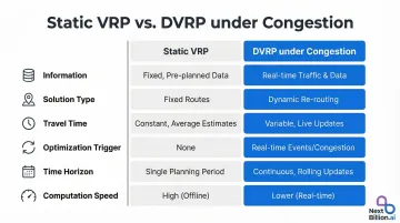
Static vs. Dynamic Routing—Key Differences
Core operational differences:
| Feature | Static VRP | DVRP under Congestion |
|---|---|---|
| Information | Deterministic input known beforehand | Stochastic input revealed dynamically |
| Solution Type | Fixed a-priori routes | Adaptive policies mapping states to actions |
| Travel Time | Constant or Euclidean distance | Time-dependent, stochastic, segment-based |
| Optimization Trigger | Single batch run | Event-driven or interval re-optimization |
| Time Horizon | Long-term planning | Near-term events weighted more heavily |
| Computation Speed | Minutes acceptable | Sub-second mandatory |
Degree of dynamism (DoD):
Not all DVRP instances are equally dynamic. DoD measures the ratio of dynamic requests to total requests. A system where 10% of orders arrive mid-route differs drastically from a taxi dispatch where 100% of trips are real-time.
Weakly dynamic systems tolerate periodic re-optimization. Strongly dynamic systems require continuous decision-making. Effective DoD (EDoD) improves measurement by capturing request urgency relative to planning horizon.
The True Operational Cost of Traffic-Blind Routing
Truck congestion costs reached $35.8 billion in 2024, accounting for 13% of total U.S. congestion costs. The commercial value of truck travel time is estimated at $80.16 per vehicle per hour, with 57% of truck delays occurring during peak periods.
The business case for traffic-aware routing is concrete. A rollout algorithm applied to a Singapore logistics company achieved a "7% improvement in total travel time" by modeling non-stationary stochastic traffic states, generating routing policies "in under 2 seconds." That translates directly to fuel savings, increased delivery capacity, and better SLA compliance.
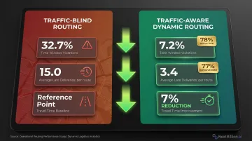
Those gains matter because congestion failures cascade fast. A single vehicle delayed 20 minutes doesn't just miss one delivery window — it compresses remaining stops, forces service violations, triggers customer complaints, and may require costly re-dispatching. In a simulated urban delivery scenario, traffic-aware dynamic routing reduced time window violation rates from 32.7% to 7.2% and decreased average late deliveries from 15.0 to 3.4.
Manual workarounds compound the problem. Operations teams relying on drivers to self-navigate around congestion — or dispatchers to manually re-sequence stops — generate hidden costs that never appear in fleet reports. Every manual intervention wastes time, creates inconsistency, and misses routing improvements that algorithms execute in milliseconds.
How the DVRP Under Congestion Is Modeled and Solved
Markov Decision Process (MDP) Framework
Because traffic congestion evolves stochastically over time, DVRP is well-suited to MDP formulation. At each "decision epoch" (when a vehicle finishes a stop), the system observes current congestion states across all arcs and selects the next destination that minimizes expected total travel cost.
Traffic congestion on individual road segments can be modeled as a non-stationary Markov chain, where transitions between congested and uncongested states carry probabilities that shift by time of day.
Since exact MDP solutions are computationally intractable at scale, practitioners use approximate methods. Rollout algorithms combine a fast heuristic (such as nearest-neighbor search) with Monte Carlo simulation to evaluate one-step lookahead decisions. This approach produces high-quality policies in under 2 seconds per decision epoch, making it practical for real operations.
When MDP-based methods can't capture the full complexity of evolving traffic patterns, machine learning offers a more adaptive alternative.
Machine Learning Approaches—Learnheuristics
Learnheuristics combine metaheuristic optimization algorithms with machine learning predictive models. In DVRP under congestion, ML models are trained on historical traffic data to predict how travel times will evolve during route execution. These predictions feed into the metaheuristic at each iteration, allowing the algorithm to anticipate congestion rather than merely react.
ML-based approaches work best when traffic patterns are complex but learnable from historical data. That said, they're not universally superior:
- Outperform traditional methods on predictable patterns: rush-hour spikes, recurrent bottlenecks
- Require sufficient historical data volume to train effectively
- Struggle with rare, non-recurrent events like accidents or sudden road closures
- Work best paired with event-driven re-routing logic to handle anomalies
For fleets operating in data-rich environments with stable traffic corridors, a hybrid approach covers both cases. For operations with less historical data or highly variable conditions, agile optimization is a more reliable fallback.
Agile Optimization for Real-Time Constraints
Agile optimization uses parallelized heuristic algorithms to produce good solutions in milliseconds. Multiple biased-randomized versions of a fast heuristic run simultaneously; the best result is returned.
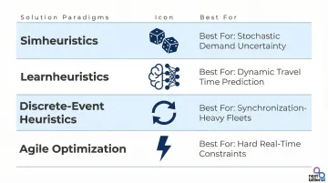
Each of the four paradigms serves a distinct use case:
| Paradigm | Best For |
|---|---|
| Simheuristics | Stochastic demand uncertainty |
| Learnheuristics | Dynamic travel time prediction |
| Discrete-event heuristics | Synchronization-heavy fleets |
| Agile optimization | Hard real-time constraints |
If your operation generates rich historical traffic data, learnheuristics will typically outperform. If sub-second response time is the hard constraint, agile optimization is the right starting point.
Practical Approaches Logistics Teams Use Today
Rolling Horizon Approach
Rather than re-optimizing the entire remaining route on every traffic update, operators set re-optimization triggers:
- Time-based: Every N minutes
- Event-based: When travel time deviation exceeds X%
Only the unexecuted portion of each route is re-optimized. Too frequent wastes compute resources; too infrequent misses congestion signals worth acting on.
That re-optimization cadence is only as good as the traffic data feeding it.
Traffic State Estimation from Multiple Sources
Modern DVRP systems ingest:
- Road sensor speed data
- GPS probe vehicles
- Connected fleet telematics
- Historical patterns
Individual arc travel times are best estimated by decomposing the arc into constituent road segments and convolving their speed distributions, which is far more accurate than treating each arc as a single unit with one travel time.
Time Window Management Under Uncertainty
In VRPTW (vehicle routing with time windows), traffic congestion creates hard conflicts—a vehicle on schedule can fall outside a customer's service window due to upstream delay.
Practical systems use soft time window constraints with penalty functions, allowing controlled violations rather than cascading infeasibility. This tradeoff is well-supported: research shows that allowing a "4.37% increase in the total transportation cost on average leads to a significant decrease in the total service cost."
Understanding which constraints can flex — and by how much — feeds directly into how you structure your decision-making process.
Operational Decision Framework
Evaluate your situation with four questions:
- What is your degree of dynamism? (% of orders/conditions changing mid-route)
- Do time windows require hard compliance or can penalties be absorbed?
- What level of re-optimization latency is acceptable?
- Do you have historical traffic data sufficient to train predictive models?
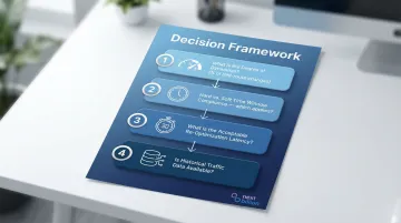
Your answers determine whether a simple re-optimization cadence, an ML-augmented system, or full agile optimization fits your operation — and where to invest first.
What to Look for in a Real-Time Route Optimization Platform
Technical Requirements for Traffic-Aware DVRP
An effective traffic-aware platform must:
- Ingest live traffic data at arc-level (not just turn-by-turn navigation)
- Support time-dependent travel time matrices that update throughout the day
- Generate re-optimized routes with sub-second latency so dispatch decisions happen before conditions change
Constraint Fidelity as a Differentiator
When congestion hits, re-routing is only half the problem. Platforms that reroute without honoring operational constraints put SLA compliance and driver hours at risk. The constraints that matter most include:
- Vehicle capacities and load limits
- Driver hours-of-service windows
- Customer delivery time windows
- Stop sequencing and priority rules
NextBillion.ai's route optimization engine enforces 50+ hard and soft constraints during dynamic re-optimization, so traffic-driven reroutes stay operationally valid — not just geographically convenient.
Integration Requirements
Dynamic routing only works if real-time vehicle positions feed back into the optimizer continuously. Look for:
- Native integrations with fleet telematics providers (Samsara, Geotab, Motive)
- APIs that push updated ETAs to customer-facing systems automatically
- On-premise deployment options for enterprises with data residency requirements
NextBillion.ai supports distance matrix computation up to 5000×5000 with live traffic processing — enough coverage for fleets managing hundreds of simultaneous routes across multiple regions.
Frequently Asked Questions
What is the difference between a static VRP and a dynamic VRP?
In a static VRP, all inputs (customers, demands, travel times) are known before routes are planned and do not change during execution. In a DVRP, information evolves in real time—new orders arrive, travel times shift with traffic—and routes are continuously updated rather than fixed in advance.
How does traffic congestion specifically affect vehicle routing optimization?
Congestion makes travel times between stops both time-dependent (varying by hour) and stochastic (unpredictable even within a time period), invalidating pre-planned routes. This forces systems to model arc travel time as a probability distribution rather than a fixed value, significantly increasing computational complexity.
What algorithms are most commonly used to solve the DVRP under traffic congestion?
Three main approaches dominate in practice:
- Markov Decision Process models with rollout algorithms for sequential decision-making
- Learnheuristics combining ML with metaheuristics for predictive routing
- Agile optimization (parallelized fast heuristics) for real-time re-routing
The best choice depends on system dynamism, data availability, and latency requirements.
How often should routes be re-optimized in a dynamic routing system?
Re-optimization can be time-triggered (every fixed interval), event-triggered (when a stop is completed, a new order arrives, or travel time deviation exceeds a threshold), or continuous. Most production systems use event-triggered approaches with minimum intervals to balance responsiveness and efficiency.
What data is required to implement traffic-aware vehicle routing?
Traffic-aware routing depends on four key data inputs:
- Real-time vehicle GPS positions
- Road-segment-level speed data (from sensors, probe vehicles, or traffic APIs)
- Historical speed patterns by time of day
- Accurate customer time windows
The more granular the road-segment data, the more precisely arc travel time distributions can be estimated.
Can machine learning replace traditional optimization algorithms in dynamic vehicle routing?
ML works best alongside optimization algorithms, not in place of them. It predicts how traffic will evolve, turning uncertain inputs into better estimates—while optimization algorithms use those estimates to generate feasible, constraint-respecting routes. Pure ML approaches lack the constraint-handling and solution quality guarantees that operational logistics requires.