Introduction
Every day, logistics fleets navigate a staggering operational puzzle: completing dozens—sometimes hundreds—of stops per shift within impossibly tight delivery windows. For a standard FedEx route averaging 75 to 125 stops per driver, the number of possible stop sequences exceeds the number of atoms in the observable universe. Manual planning simply cannot compute these combinations, making this an operationally critical challenge across e-commerce distribution, field service, and last-mile logistics.
The financial stakes compound the complexity. Deloitte reports that last-mile operations account for 30% to 35% of total delivery costs, with inefficient routing eroding margins through wasted fuel, excess driver hours, and missed windows.
When routes fail, the consequences cascade: up to 20% of e-commerce packages fail on the first delivery attempt, triggering costly redeliveries and customer churn.
This guide explains how logistics teams actually execute multi-stop route optimization—from gathering delivery inputs to running algorithmic sequencing, applying operational constraints, and monitoring real-time execution. By the end, you'll have a clear picture of where the biggest efficiency gains are hidden—and how modern optimization tools unlock them.
TL;DR
- Multi-stop route optimization finds the most efficient stop sequence for a fleet — accounting for time, distance, cost, and real-world constraints simultaneously
- Logistics teams work through a structured process: load delivery data, run optimization algorithms, apply operational constraints, then monitor routes as they execute
- The core challenge is a variant of the Vehicle Routing Problem (VRP), requiring computational optimization to solve at any meaningful scale
- Key constraints include time windows, vehicle capacity, driver shift rules, delivery types, and road restrictions
- What separates intelligent optimization from basic planning: it handles deep constraint logic, adapts to disruptions mid-route, and re-optimizes without manual intervention
What Is Multi-Stop Delivery Route Optimization?
Multi-stop delivery route optimization is the computational and operational process of determining the most time- and cost-efficient sequence, path, and resource assignment for vehicles completing multiple delivery or service stops in a single trip. It addresses a fundamental operational gap: as stop counts increase, the possible combinations of stop sequences grow exponentially—a mathematical complexity known as factorial growth. For a route with just 10 stops, there are over 3.6 million possible sequences. At 20 stops, that number exceeds 2.4 quintillion.
This combinatorial explosion makes manual or intuition-based planning inadequate beyond a handful of stops. The underlying mathematical challenge is called the Vehicle Routing Problem (VRP), first introduced by George Dantzig and John Ramser in 1959.
The VRP asks: what routes should a fleet of vehicles take to reach all customers at minimum cost? Because the VRP is classified as NP-hard—meaning no known algorithm can find the perfect solution in polynomial time—modern systems use heuristics to find near-optimal solutions quickly.
What multi-stop route optimization is NOT:
- Simply GPS navigation between pre-set stops
- The same as route planning, which defines stops without solving for optimal order or load distribution
- Single-vehicle, single-destination dispatch
Early solutions relied on static, pre-planned routes calculated the night before. Today's systems layer in real-time traffic, dynamic demand, constraint-based sequencing, and machine learning—recalculating routes as conditions shift throughout the day rather than locking in a plan at midnight.
How Logistics Teams Optimize Multi-Stop Routes
Multi-stop route optimization follows a structured workflow. Each stage depends on the quality of data and constraint logic feeding into it, and weaknesses at any point create downstream failures that no algorithm can correct.
Defining the Problem: Inputs and Delivery Data
The process begins with aggregating all inputs required to build a feasible route plan:
- Delivery addresses and geocoded locations
- Order volumes, weights, and dimensions
- Time windows (earliest and latest acceptable arrival times)
- Vehicle availability and specifications
- Driver shift start and end times
- Special handling requirements (refrigerated goods, signature-required deliveries, hazmat restrictions)
Incomplete address data, missing time windows, or unaccounted vehicle restrictions at this stage create errors no algorithm can correct. Many logistics teams use order management systems and Transportation Management System (TMS) integrations to automate this data collection, reducing manual entry errors and ensuring consistency.
Algorithmic Sequencing: Solving the Routing Problem
Routing software frames this as a Vehicle Routing Problem (VRP) or one of its variants:
- Capacitated VRP (CVRP): Vehicles have limited carrying capacity (weight or volume) that cannot be exceeded by the total demand of assigned stops
- VRP with Time Windows (VRPTW): Deliveries must occur within specific time intervals; vehicles arriving early must wait, and arriving late violates constraints
Solving these VRP variants exactly becomes computationally impractical at scale — so modern systems use heuristic or meta-heuristic algorithms to find near-optimal solutions within seconds. These include:
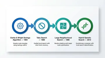
- Clarke and Wright savings algorithm (1964): Foundational heuristic
- Tabu Search (1989): Prevents revisiting recently explored solutions
- Large Neighborhood Search (LNS) (1998): Destroys and reconstructs portions of routes
- Hybrid Genetic Search (HGS) (2012): Combines evolutionary algorithms with local search
Modern enterprise optimization engines can process instances with 1,000+ customers in minutes. For example, PyVRP achieved a mean gap of just 0.40% from the Best Known Solution on 1,000-customer instances within a two-hour optimization window, demonstrating that high-quality solutions are achievable at scale.
Applying Constraints: Hard Rules and Soft Preferences
Logistics teams apply two categories of constraints:
Hard constraints (must be satisfied):
- Time-sensitive deliveries within defined windows
- Vehicle load limits cannot be exceeded
- Driver Hours of Service (HOS) regulations
- Vehicle clearance restrictions (bridge heights, weight limits)
Soft constraints (should be respected where possible):
- Minimize toll roads
- Avoid left turns (UPS famously saves millions annually with this rule)
- Group stops by geographic zone
- Prioritize high-value deliveries early in the route
The interaction between multiple simultaneous constraints is where optimization complexity lives. Adding more constraints narrows the feasible solution space, forcing trade-offs: honoring a tight time window may require a less fuel-efficient detour, while prioritizing a high-value delivery may break geographic clustering.
Handling these trade-offs at scale requires an engine built for it. NextBillion.ai's route optimization API supports 50+ hard and soft constraints and handles large-scale distance matrix computation without the stop-count limits common in standard tools — letting logistics teams model real operational rules without simplifying them away.
Dispatching and Monitoring Execution
Once routes are generated, the dispatch phase:
- Assigns routes to specific drivers and vehicles
- Pushes turn-by-turn navigation to driver apps
- Feeds expected ETAs back into customer-facing tracking systems
From there, the monitoring layer tracks live progress against the plan. When stops run long, traffic delays build, or time windows are missed, dispatchers get flagged before problems cascade.
Intelligent systems go further — triggering automatic re-optimization of remaining stops mid-route rather than waiting for a dispatcher to intervene manually. This closes the loop between planning and execution, making the entire workflow responsive to real-world conditions rather than just the ones anticipated at dispatch.
The Constraints That Shape Every Multi-Stop Route Plan
Route optimization is only valuable if the routes it produces are legal, physically possible to drive, and aligned with business priorities. Five constraint categories determine whether a plan holds up in the real world.
Time Window Constraints
Each stop may have an earliest and latest acceptable arrival time (soft or hard). Route plans must sequence stops in an order that allows drivers to satisfy all windows without excessive idle time between stops. Violating time windows directly affects SLA compliance and customer satisfaction. In 3PL contracts, SLA violations can trigger penalties of 1% to 2% of a purchase order's value per day of delay.
Vehicle Capacity and Load Constraints
Routes must account for the total weight, volume, or item count a vehicle can carry per trip. For routes with multiple stops, this also involves understanding unloading sequence: items to be delivered last must be loaded first. Errors here cause time-consuming reloading and delay cascades that ripple through the entire schedule.
Driver and Shift Rule Constraints
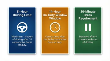
Logistics teams must respect Hours of Service (HOS) regulations, mandatory break periods, shift start and end locations, and per-driver skill or equipment certifications. In the U.S., the Federal Motor Carrier Safety Administration (FMCSA) enforces HOS rules including:
- 11-hour driving limit: Drivers may drive a maximum of 11 hours after 10 consecutive hours off duty
- 14-hour on-duty window: Drivers cannot drive after the 14th consecutive hour after coming on duty
- 30-minute break requirement: After 8 cumulative hours of driving
Failing to account for these at the planning stage creates compliance risk and unpredictable mid-route changes.
Road and Vehicle-Type Restrictions
Certain roads prohibit trucks by height, weight, or axle configuration. Under 23 CFR Part 658, federal weight limits on the Interstate System are capped at 80,000 pounds gross vehicle weight. Time-of-day restrictions in urban zones (congestion pricing windows, loading zone access hours) further constrain viable paths.
Truck-compliant routing, which factors in bridge clearances, hazmat restrictions, and vehicle-specific road rules, is a distinct requirement from standard passenger-car navigation. A 40-ton truck restricted to certain roads and bridges covers a measurably different reachable area in the same 30-minute window than a delivery van.
Prioritization Logic
High-value, time-critical, or perishable deliveries may need to be served early in the route regardless of geographic efficiency. This requires the optimizer to hold geographic clustering in tension with delivery priority ranking, creating trade-offs between distance minimization and service-level commitments.
Where Multi-Stop Route Optimization Has the Greatest Operational Impact
Last-Mile and Final-Mile Delivery
The last segment of delivery—from local hub to end customer—accounts for a disproportionate share of total logistics costs. Deloitte reports that last-mile delivery accounts for 30% to 35% of total delivery costs. Multi-stop optimization directly reduces cost-per-drop by increasing stop density per route.
Real-world deployments demonstrate massive savings:
- UPS ORION: The On-Road Integrated Optimization and Navigation system reduces each route by 6 to 8 miles, saving 10 million gallons of fuel annually
- Amazon: By optimizing regional fulfillment and routing networks, Amazon avoided nearly 16 million miles driven in 2023
Field Service and On-Demand Operations
In field service (pest control, utilities, HVAC, NEMT), optimization addresses service windows rather than delivery windows, often with unpredictable job durations. This lets dispatchers sequence technician stops to minimize drive time while absorbing schedule variability without cascade delays.
The average First-Time Fix Rate (FTFR) in field service hovers around 80%; dropping below 70% adversely affects customer retention. Optimization improves FTFR by ensuring technicians arrive on time with the right parts and sufficient time budgets.
For example, Orkin Pest Control used GPS and route consolidation software to enforce speed limits and reduce idling, saving over $3.5 million in auto liability and damage claims.
Distribution and B2B Delivery
In food and beverage distribution, manufacturing parts delivery, and other B2B contexts, routes often involve recurring stops with predictable patterns. Route efficiency gains compound across hundreds of weekly trips, creating sustained cost savings and capacity growth. AB InBev, for instance, applies route optimization across its distribution network to reduce driver hours and improve on-time delivery to retail accounts. Common gains in recurring B2B routes include:
- Lower fuel spend through tighter stop sequencing
- Increased stops per driver per day without extending shift hours
- Faster reintegration of new accounts into existing route structures
What Separates Basic Route Planning from Intelligent Optimization
The Functional Gap
A basic route planner finds a path between pre-set stops, typically with limited stop count and constraint support. An enterprise-grade optimization engine solves VRP variants at scale, supports dozens of operational constraints simultaneously, and re-optimizes dynamically as conditions change.
Stop-Count Limitations:
| Routing Tool / API | Stop-Count Limitation | Best Fit |
|---|---|---|
| Google Routes API | Maximum 25 intermediate waypoints per request | Prototyping, small local fleets |
| Mapbox Optimization API v2 | Maximum 1,000 locations per routing problem | Mid-market batch routing |
| Enterprise VRP Solvers | 1,000 to 10,000+ customers | High-volume enterprise logistics |
Buyers must ensure the underlying engine can handle their peak daily order volume in a single batch, rather than relying on APIs that cap at 25 waypoints.
Dynamic Re-Optimization
When a driver is delayed, a stop is cancelled, or traffic creates a deviation, an intelligent system can recalculate the optimal sequence for remaining stops in real time—rather than requiring dispatchers to manually reroute. Sub-second response times matter here: delays in re-optimization translate directly into cascading SLA risk.
Research on the Dynamic Delayed Time Window Assignment VRP found that strategically delaying time window assignments to allow the algorithm more time to optimize can decrease routing durations by 11.82%, with only marginal increases in routing costs.
Pricing Model Differences
Capability differences only matter if the pricing model holds up at scale. Buyers must align the pricing structure with their operational volume before committing to a platform:
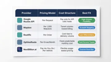
| Provider | Pricing Model | Cost Structure |
|---|---|---|
| Google Routes API | Per-Request / Per-Element | Pay-as-you-go based on features used; matrix requests billed per element (origins × destinations) |
| Mapbox | Per 1,000 Requests | Tiered pricing (e.g., $2.00 per 1,000 requests for Optimization API) |
| Routific | Per-Order | Flat monthly fee ($150) up to 1,000 orders, plus per-order fee for higher volumes |
| OptimoRoute | Per-Driver / Month | Flat fee per driver (e.g., $35.10 to $44.10/mo billed annually) |
| NextBillion.ai | Pay-as-you-go / Per-Vehicle | Scales with operational volume; per-vehicle or per-order options available |
Fleets with high order volumes but few drivers benefit from per-driver pricing. Operations with variable gig-fleets are better served by per-order or task-based models, where costs track actual activity rather than fixed headcount.
Frequently Asked Questions
How to optimize a route with multiple stops?
Define all stop locations, time windows, and vehicle constraints as inputs, then run a VRP solver to determine the most efficient stop sequence. Unlike manual sequencing, optimization algorithms evaluate millions of possible combinations to find near-optimal solutions in seconds.
What is the difference between route planning and route optimization?
Route planning defines where to go—stops, waypoints, and paths. Route optimization determines the best possible order and assignment of those stops across one or more vehicles, factoring in constraints like time windows, capacity, and driver rules. Planning is a subset of optimization.
What is the Vehicle Routing Problem (VRP) in logistics?
VRP is the mathematical problem of finding optimal routes for a fleet to serve a set of locations. It becomes computationally complex at scale (NP-hard), so logistics software uses heuristic algorithms to reach near-optimal solutions quickly instead of computing the perfect answer.
What constraints do logistics teams typically apply to multi-stop routes?
Main categories include time windows (delivery deadlines), vehicle capacity (weight/volume limits), driver hours (HOS/shift rules), road restrictions (truck-specific routing), and delivery priority. Hard constraints must be satisfied; soft constraints should be respected where possible.
How does real-time traffic affect multi-stop route optimization?
When delays are detected, the system recalculates the remaining stop sequence in real time, updating ETAs and reordering stops to protect SLA compliance and overall route efficiency.
How long does it take to optimize a multi-stop delivery route?
Modern enterprise optimization engines can generate optimized routes for hundreds or thousands of stops in seconds to a few minutes, depending on fleet size and constraint complexity. This contrasts sharply with the hours required for manual planning at equivalent scale.
Ready to optimize your multi-stop delivery routes? NextBillion.ai's Route Optimization API supports 50+ hard and soft constraints, handles large-scale distance matrix computation without stop-count limitations, and connects directly with fleet management platforms like Samsara, Geotab, and Motive. Contact our team to see what's possible at your scale.